1. Click on Animation on the homepage to bring up the Applet.
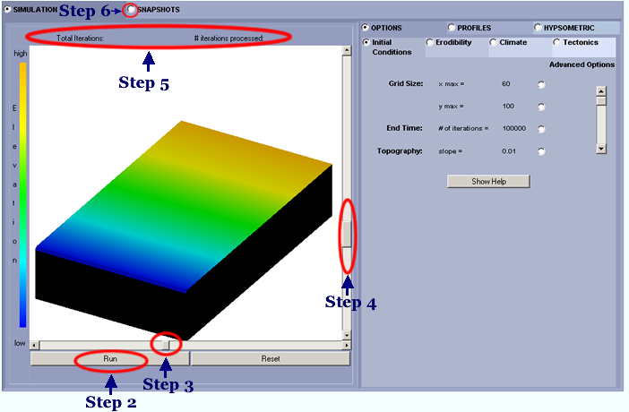
2. This
scenario of constant erodibility, constant climate and no tectonic
uplift is the default. So there is no need to change
any parameters. Simply click on the Run button as pointed by the
step 2 arrow shown in the above figure to start the simulation.
3. You can click on the horizontal bar (as pointed
by the step 3 arrow in the above figure) and drag it to different
horizontal position to change the azimuth angle of viewing.
4. You can click on the vertical bar (as pointed
by the step 4 arrow in the above figure) and drag it to different
vertical position to change the elevation angle of viewing.
5. The total number of iteration and current iteration
will be shown in the area pointed by step 5 arrow.
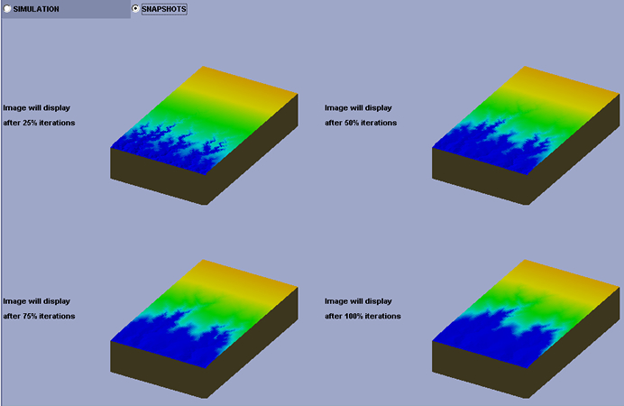
6. Click on the Snapshots tab to see the still
images at every 25% iterations.
Branching channel networks are developing and extending headward.
Note
your simulation
may
not
look exactly like the figure shown here due to the randomness
in the model.


1. In
this scenario, the erodibility changes (or there is an erodibility
break) at row 15 (y = 15). The erodibility for rows 15 and
above is 0.04 and that for rows below 15 is 0.01.
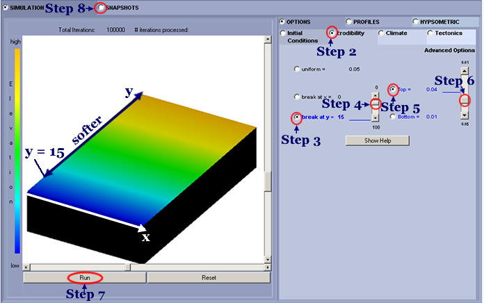
2. Click
on the Erodibility Tab as pointed by step 2 arrow.
3. Click on the radio button next to "break
at y" as pointed by step 3 arrow.
4. Click
on the slide bar as pointed by step 4 arrow and drag it down until
the y value is equal to 15.
5. Click
on Top radio button as pointed by step 5 arrow.
6. Click
on the slide bar as pointed by steps 6 arrow and drag it down until
the erodibility value next to the Top button is equal to 0.04.
7. Click
on the Run button as pointed by step 7 arrow to run the model.
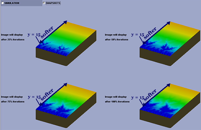
8. Click
on the Snapshots tab to see the still images at every 25% iterations. Branching channel networks are developing and extending
headward. As the erosion gets into the softer part
of the terrain (higher erodibility), the shape of the channel looks
fuzzier as compared to the hard part of the terrain (lower erodibility).
Note your simulation may not look exactly like this one due to
the randomness in the model.

1. In
this scenario, everything stays as default except that there will be tectonic
uplift for rows 40 and above. In essence, this scenario simulates a vertical
fault at row 40 (y = 40).
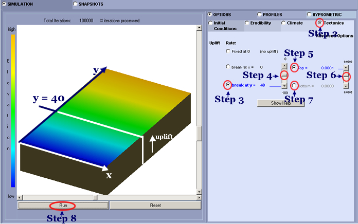
2. Click
on Tectonics tab as pointed by step 2 arrow.
3. Click the radio button next to “break
at y” as pointed by step 3 arrow.
4. Click on the slide bar as pointed by step 4 arrow
and drag it to the right until the y value is equal to 40.
5. Click on Top button as pointed
by step 5 arrow.
6. Click on the slide bar as pointed by step 6 arrow
and drag it down until the uplift rate value next
to the Top button is equal to 0.0001.
7. The Bottom button
will be disabled as pointed by Step 7 arrow.
8. Click on the Run button to
run the model.
The user may also do any of the following steps as he/she wishes:
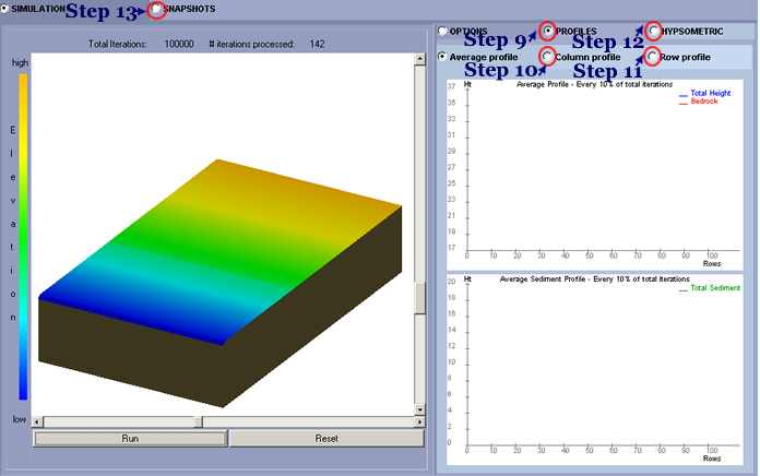
9. To see the profiles, click on Profiles tab. To see the
average profile, do nothing (this is the default). The profiles will be
displayed at every 10% of the total iterations.
10.To see the column profiles click on the Column
Profile subtab
and drag the slider to select a column value. Profiles will be displayed at every
10% of the total iterations.
11.To see the row profiles click on the Row Profile subtab
and drag the slider to select a row value. Profiles will be displayed
at every 10% of the
total iterations.
12.To see the hypsometric curves, click
on the Hypsometric tab. Hypsometric curves will be displayed
at every 10% of
the total iterations.
13.Click on the Snapshots tab to see the still
images at every 25% iterations.
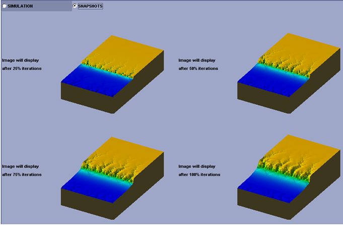
Branching channel networks are developing and extending
headward in the stable portion of the terrain as previous scenarios.
Alluvial fans are developing along the boundary between the stable
and uplifting parts of the terrain. Branching channel networks
are also developing and extending headward on the uplifted plateau.
Note your simulation may not look exactly like this one due to
the randomness
in the model.

1. In
this scenario, all parameters are the same as scenario 3 except the
climate is changing from wet to dry.
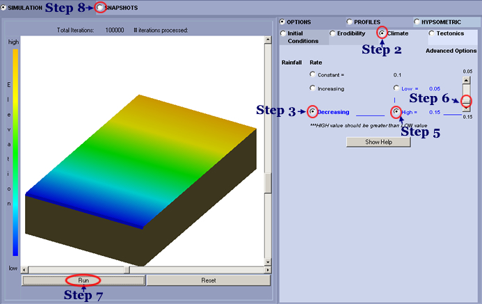
2. Click on the Climate tab
as pointed by step 2 arrow.
3. Click on the radio button next to “Decreasing” as
pointed by step 3 arrow.
4. Keep the default Low value 0.05.
5. Click on the radio button next to "High"
as pointed by step 5 arrow.
6. Click
on the slide bar pointed by step 6 arrow and drag it down until
the High value is equal to 0.15.
7. Click
on the Run button to run the simulation.
8. Click on the Snapshots tab
to see the still images at every 25% iterations. Branching channel
networks are developing and extending headward. Alluvial
fans are developing initially but do not grow much as the climate
turns drier and diffusive process starts to dominate. The final
landform looks very smooth due to the dominance of diffusive
process in an increasingly drier climate. Note your simulation may
not
look exactly like this one due to the randomness in
the model.

