We assume that you have worked with the linear version of the model and are familiar with how cellular automata algorithm works [if not, please see How It Works under Beginning User (Linear Version) tab]. The linear version of WILSIM is simple and easy to implement. However, it does not explicitly simulate the nonlinear behavior of sediment erosion and transportation and precludes the simulation of interactions between precipitons (i.e., each precipiton, or storm event, is independent of any other precipiton).
1. The nonlinear rules
In the nonlinear version of the model, the amount of erosion is calculated as follows:
 (1)
(1)
where  is the maximum possible erosion;
e is the erodibility of material in current cell;
s is local slope of current cell;
a is contributing area to current cell;
m and n are exponent coefficients.
2. How to Determine the Contributing Area a
The contributing area of a cell is defined here as the number of cells flowing into that cell. In the implementation, before each iteration of erosion and deposition of a precipiton starts, the program loops through the grids twice: the first time to determine the flow direction of each cell by finding the lowest neighboring cell of each cell, and the second time to follow the flow direction and sum up the number of cells that flow into each cell (i.e., the a in equation (1) ).
To further illustrate how this works, a schematic 5×5 example and its resultant flow direction grid and contributing area grid are shown below ( indicates sink).

For instance, for cell A1, it has 3 neighboring cells (A2, B1 and B2) and the lowest of them is B1, so the flow direction is south (downward). For cell C3, the lowest of its 8 neighboring cells is D2, so the flow direction is southwest (to lower left). You can verify the rest of the flow directions. After the flow direction is determined, the program runs through the grid cells again to count how many cells flow into each cell according to the flow direction. For instance, for cell A1, it has only one contributing cell, itself, so its contributing area a = 1. For B1, it has A1 and A2 flowing into it, plus itself, so its contributing area a = 1 + 1 + 1 = 3. For cell C2, it has B1, B2, and B3 flowing into it, so the contributing area of cell C2 is equal to the sum of contributing areas of B1 (3), B2 (2), and B3 (1) plus that of itself (1), a = 3 + 2 + 1 + 1 = 7. Please verify the rest of the contributing area yourself. Also notice that the contributing area of the two sinks add up to the total number of cells of the grid (14 + 11 = 25). This method is commonly known as D8 algorithm ( O'Callaghan and Mark, 1984; Jenson and Domingue, 1988).
Once the flow direction and contributing area for each cell are determined, a precipiton is randomly dropped onto the grid and it moves downhill according to flow direction and conduct erosion and deposition along the way as in the linear case except the amount of erosion is governed by equation (1). Before a new precipiton is dropped, the flow direction and contributing area need to be updated as the erosion and deposition from current precipiton can change the elevation and thus change the flow direction and contributing area. So this is a computationally extensive process.
By incorporating the contributing area into the calculation of erosion, the precipitons are no long independent, as larger contributing area of a cell is usually caused by more erosion from previous precipitons. This is similar to social insects such as ants leaving a chemical pheromone trail, which is read by other ants who arrive later and adjust their behavior accordingly (for example by following the path) (Haff, 2001).
When m = n = 1, the amount of erosion is essentially the same as the linear case. In other words, everything that can be done in the linear version can be done in the nonlinear version. However, the linear model will be faster since it simply deals with a 3×3 local neighborhood and does not require the two additional loops before each iteration to determine flow direction and contributing area as in the nonlinear case.
What's New in the Graphical User Interface (GUI)?
1. The Exponent Coefficients m and n
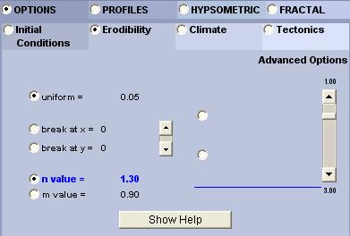
The nonlinear exponent m and n is located under under OPTIONS tab, Erodilibty subtab. The default values for m and n are 1.2. To change the default value, click on the button next to n value or m value and drag the slider to the right as shown below.
2. Fractal Dimension
To show the changes in roughness of the topographic surface as it evolves over time, we added the FRACTAL tab to display a graph of fractal dimension. Simply speaking, fractal dimension is a number used to measure the roughness of an object. For a 2-D line, the fractal dimension ranges between 1 (a point) and 2 (space filling line, a line so jagged that it fills the 2-D plane). For a 3-D surface the fractal dimension ranges between 2 (a perfect plane) and 3 (a space filling surface). In general, the larger the fractal dimension value, the rougher the surface. The fractal dimension presented here is computed using the cubic covering method developed by Zhou and Xie (2003). It is displayed at every 10% of the total iterations.
Example Results
Figure 1 shows the snapshot of a simulation with n = 1.2, m = 1.2 and tectonic uplift. Comparing with the linear simulation (Figure 2, n = 1 and m = 1), the nonlinear model is much rougher and the channel networks extend much further upstream. This is also shown in their respective fractal dimension plots (Figures 3).
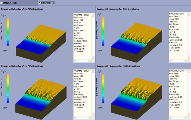
Figure 1
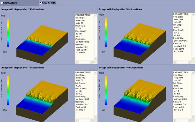
Figure 2
Figure 3. Left: fractal dimension of nonlinear model (figure 1); Right: fractal dimension of linear model (figure 2).
References Cited
Haff, P. K., 2001, Waterbots, in Landscape Erosion and Evolution Modeling , edited by Harmon R. S. and Doe, W. W. III, Kluwer Academic/Plenum Publishers, New York, p. 239-275.
Jenson, S.K. and Domingue, J.O., 1988, Extracting topographic structure from digital elevation data for geographic information system analysis, Photogrammetric Engineering and Remote Sensing , 54(11), 1593-1600.
O'Callaghan, J.F. and Mark, D.M., 1984, The extraction of drainage networks from digital elevation data, Computer Vision, Graphics, and Image Process. , 28(3), 323-344.
Zhou, H.W. and H. Xie, 2003, Direct estimation of the fractal dimensions of a fracture surface of rock, Surface Review and Letters , 10(5), 751-762.
(http://www.worldscinet.com/srl/10/preserved-docs/1005/S0218625X03005591.pdf )
