
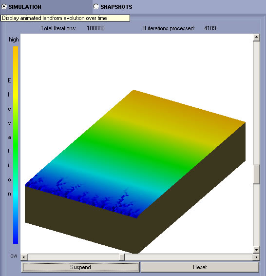
This is the default main display
window that dynamically shows the animated landform evolution over
time. The slide bars are used to control the viewing angle. The vertical
bar
controls
elevation
angle
and the
horizontal bar controls the azimuth
angle. The Run button is used to start and suspend the animation.
The simulation will start from the initial condition. The Reset
button is used to reset the values and continue the animation. You
can suspend the simulation, adjust the parameters and then continue
the simulation.
The simulation will continue from where it paused.

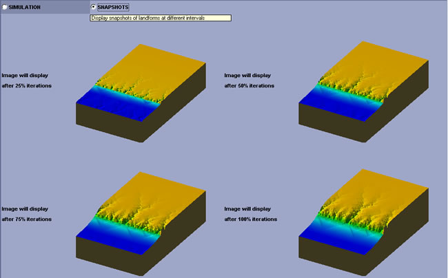
This tab displays snapshots of landforms
different time intervals (at every 25% of the total iterations). This
allows the user to compare still images of the landform at different
stages of development.

This tab allows user select various
parameters that control the simulation. There are 4 subtabs: Initial
Conditions, Erodibility, Climate, and Tectonics.

Under this subtab, you can change
the following parameters related to initial model conditions:
Grid size:the
number of columns (x) and rows (y) of the grid. The default is
60x100. You can change each by clicking on the radio buttons on
the right of each option and selecting
a value using the slide bar.
End time: the maximum number of iterations you want this simulation
to run. The default is 100,000. You can adjust this value by clicking
on the radio button on the right of this option
and selecting a value using the slide bar.
Topography: you
can adjust the slope of the initial topographic grid. The default
is 0.01 slope. You can adjust this value by clicking
on the radio button on the right of this option and selecting
a value using the slide bar. (Note: a very small amount of random
roughness
is added in the initial topography to simulate natural surface
and to avoid precipiton running downhill along straight lines)

Erodibility: the
erodibility of the bedrock. This parameter controls how easy the
bedrock will be eroded. There are 3 options:
(1)uniform:0.05,
each cell has the same erodibility of 0.05. This is the default
value but it can be changed by selecting its radio
button and using the slide bar.
(2)break at x: meaning
the erodibility changes at a column (x) specified by user
with the slide
bar. The actual erodibility on either side of the break
line is specified by clicking on the left and right button
and selecting a value using the slide bar.
(3)break at y: similar to break at x except that the change will occur
at a row (y) specified by user.

This tab is used to control the amount of rainfall
over time. There are three options:
(1)Constant rainfall: meaning the amount of rainfall will
be constant over time. The default value is 0.10. You can also
adjust this value by clicking on the button and select a value using the
slide bar.
(2)Increasing rainfall: meaning the rainfall will increase
linearly over the time period of your simulation. You can specify
the low end and the high end of the linear function by clicking on the
Low and High radio button and selecting a value using the slide
bar.
(3)Decreasing rainfall:meaning
the rainfall will decrease linearly over the time period of your
simulation. The high and low end of the linear function can be
changed similarly.

This tab allows you to change the tectonic uplift
rate. The uplift is applied to the topographic grid after each iteration.
There are three options:
(1)Fixed at 0 (no uplift): meaning the uplift rate will be 0 (i.e.,
no uplift). This is the default.
(2)Break at x: meaning the uplift rate changes at a column
(x) specified by user with the slide bar. The actual uplift rate
on one side of the break line is specified by clicking on the
"Left" or "Right" radio buttons and selecting a value using the
slide bar. The other side is fixed at 0 (no uplift).
(3)Break at y: similar to break at x, except that the change will
occur at a row (y) specified by user.

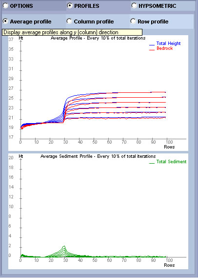
This tab displays profiles (or cross-sections) of
the landform at different time intervals. There are 3 subtabs: Average Profile,
Column Profile, and Row Profile

This subtab displays average profiles along y (column)
direction (i.e., the elevation at each row is the average of all the cells at that row).
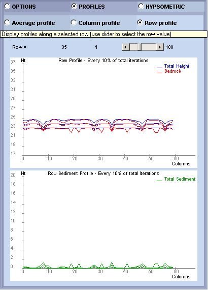
The top panel displays the surface elevation (total height in blue) and bedrock
elevation (bedrock in red). The bottom panel displays the sediment depth (the difference
between surface elevation and bedrock elevation). The profiles are displayed at every 10%
of the total iterations.

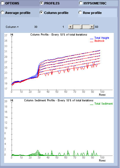
This subtab displays the profile of one individual column
selected by the user. Other features of the profile are similar to the average profile.

This subtab displays the profile
of one individual row selected by the user. Other features of the
profile are similar to the average profile.

This tab displays the hypsometric
curve of the whole model topographic grid at every 10% of the total
iterations. The hypsometric curve displayed here is slightly different
from the traditional hypsometric curve in that it is defined for
the whole model tropographic grid, not a watershed.
Continue to read about a Tutorial
with step by step instruction for simulating different scenarios.
 References
Cited
References
Cited
Ahnert, F., 1987, Approaches to dynamic equilibrium in theoretical
simulations of slope development, Earth surface processes and landform,
v. 12, p. 3-15.
Chase, C. G., 1992, Fluvial landsculpting and the fractal dimension
of topography, Geomorphology, v. 5, p. 39-57.
Howard, A. D., 1994, A detachment-limited model of drainage basin
evolution, Water Resources Research, v. 30, p.2261-2285.
Willgoose, g., Bras, R.L., and Rodriguez-Iturbe, I., 1991, A coupled
channel network growth and hillslope evolution model, 1. Theory,
Water Resources Research, v. 27, p.1671-1684.

 Figure
3
Figure
3