As an example, let's just edit the run_card.dat, so that we'll generate 5000 events at the LHC with center-of-mass energy 8 TeV, which was the energy of the last run. To do this, type
-
2
Now on line 32 change "10000 = nevents" to "5000 = nevents",
and on line 41 change "6500 = ebeam1" to "4000 = ebeam1",
and on line 42 change "6500 = ebeam2" to "4000 = ebeam1".
Energies and masses are always in GeV. Then save and quit the editor (control X if you are using pico).
We won't edit any of the other cards this time, so now back at the Madgraph prompt, type:
-
0
Looking at the results
When the event generation and detector simulation are done, you will see something like:
=== Results Summary for run: run_01 tag: tag_1 ===
Cross-section : 134.3 +- 0.339 pb
Nb of events : 5000
This confirms that you generated 5000 events, and tells you what the total cross-section was for the process or processes that you selected. Warning: don't take the uncertainty of +- 0.339 pb seriously. At best, this is statistical uncertainty only, and the systematic uncertainty is always much higher.
When the Madgraph prompt returns, you are ready to look at the results of the run. Issue the command:
-
open index.html
Plots at parton level:
First, click on the plots link in the row that is labelled "parton madevent". You should see a page with lots of histogram plots. The first one is a plot of weights, which is trivial; the weights are always just 1. The second plot is just a histogram of the number of top quarks. This is also trivial in this case, because every event you generated had exactly one top quark. The third plot is a histogram of the number of antitop quarks, which is also trivial for the same reason.The next plot, of "Ecm", the center of mass energy, of the partonic collision is more interesting. It should look something like this:
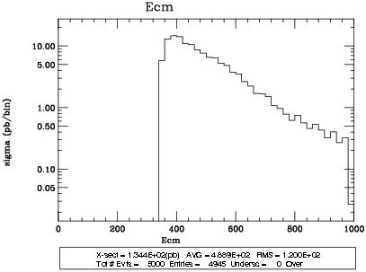
Note that Ecm has to be at least twice the top quark mass, so greater than 2 * 173 = 346 GeV. The Ecm is usually not much more that that, however, because the probability to find a parton with a given energy decreases sharply with the energy. There is a long tail at higher energies.
Scrolling farther down, "pt(t1)" and "pt(t~1)" are the momentum transverse to the beam direction for the top and antitop quarks respectively. The graph of the transverse momentum of the top quark should look something like this:
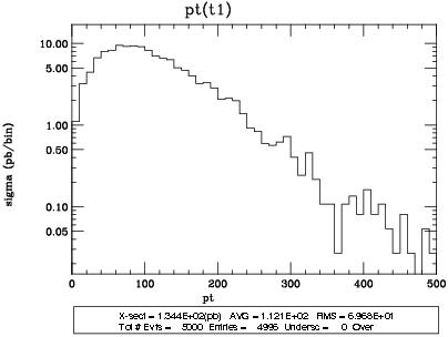
We can see that it is peaked from about 50 to 100 GeV. The graph of the transverse momentum of the antitop quark looks identical. That's because they are produced back-to-back in the center-of-mass reference frame.
The last plot is of "m(t1,t~1)" which is the invariant mass of the top+antitop pair. The invariant mass is the mass of a single particle that could have decayed to those two partons, even if no such particle exists. In real data, if you see a strong peak in m(i,j), it might mean that such a particle does exist, and you discovered it. For just two partons, (top and antitop here), the invariant mass is the same as the partonic center-of-mass energy. It therefore looks the same as the Ecm plot above, except it is produced with different axis scales.
Plots at detector level, using DELPHES:
Before looking at some of these, note that there are very similar plots
produced by PGS, and by Pythia. You can compare them and try to figure
out the differences, which are often very slight. They each reconstruct
jets and other objects in
different ways, so it is expected that they don't agree with each other
perfectly. But, for brevity, let's stick to the DELPHES results only.
The DELPHES detector simulator reconstructs "objects" in each event
as the following:
For each event, the objects of a given type (other than MET) are numbered in order of decreasing transverse momentum, pT. Thus "j1" means the jet that has the largest pT, "j2" has the second-largest pT, etc. This also applies to the lists of b-jets, electrons, muons, taus, and photons.
The histogram of the number of jets looks like:
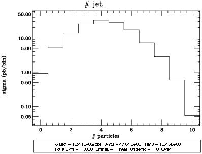
We see that the most probable number of jets as reconstructed by DELPHES is 4, but there could be 0 or as many as 10.
For b-jets:
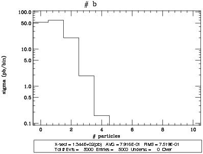
In principle, there "should" be 2 b-jets in each event. However, often one or both of the b-jets is not tagged. The most likely number of b-tags turns out to be 1 in this process. Also, note that occasionally 3 jets are b-tagged, even though there "should" only be 2. That is partly because the detector simulator has a small mistagging probability built into it, just like in the real world. Another source of additional b-tags is that a parton can radiate off another bottom-antibottom pair when hadronization occurs in the final state.
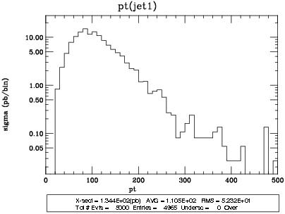
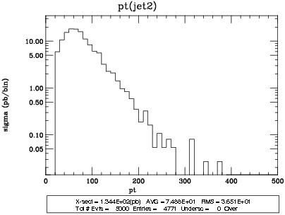
Here are the plots of the pT of j1 and j2, the leading and sub-leading jets:
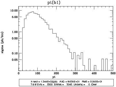
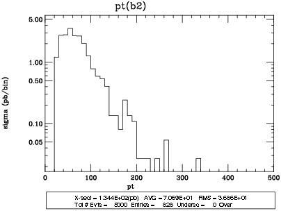
and the same for the leading and sub-leading b-jets:
Here is the invariant mass m(b1,b2) of the leading two b-jets, b1 and b2:
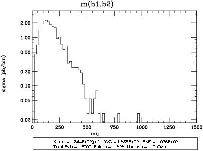
This may look like it has a broad peak-like structure. But, remember that a b-jet would not be reconstructed at all if the energy were too small. So that means that there can't be many events with small m(b1,b2). And, kinematics makes it unlikely also to have very energetic partons, so there can't be too many events with large m(b1,b2), either. So somewhere in between, there is a "peak". But this does not mean that some new particle decayed to b1 and b2 in these events! Separating real peaks from "fake" peaks is an important skill.
Here is the histogram of the Missing ET:
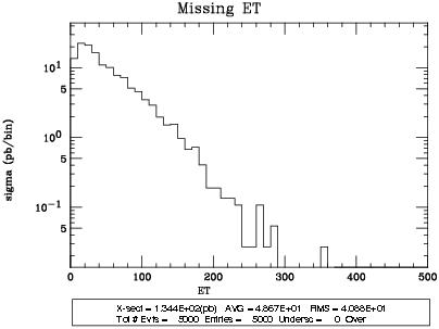
The MET has a large tail at high values. This is mostly due to the presence of neutrinos in the event. It is also partly due to mismeasurements of jet energies, which lead to "fake" missing energy.
Finally, here is the histogram of the kinematic quantity HT, which is defined to be the sum of the pT's of all of the jets, leptons, and photons in the event, plus the Missing ET:
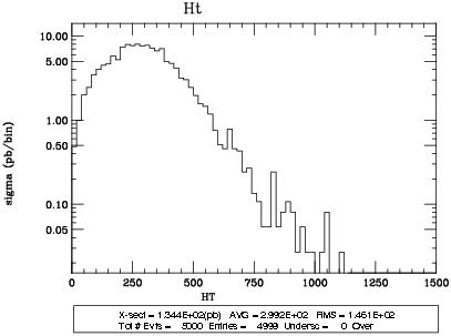
This quantity is often taken as a measure of the overall mass scale of the event. If you produce heavy particles, they are more like to give events with large HT.
By default, there are many other plots produced, including: pT's of every particle type, pseudo-rapidities of every particle type, invariant masses of every pair of particle type, distances and angles between pairs of particles.
You can also analyze the output files from Pythia, PGS or Delphes to make your own plots of kinematic quantities of interest. That's an advanced topic that we won't go into in this class, but it is essential if you end up doing your own analyses later. You can find those output files, compressed by gzip, in the directory: /xdata/$USER/madgraph/MY_FIRST_MG5_RUN/Events/run_01 .
To continue learning about the basic Madgraph capabilities, continue here: http://www.niu.edu/spmartin/madgraph/madsyntax.html.