Adding another process
Often, one wants to combine more than one process in the same event
sample. For example, you can do combined top and bottom production:
Now you can output the resulting combined processes:
The resulting events generated will be correctly weighted according to their individual cross-sections. This time we will only be interested in the cross-sections, and not want to look at plots of kinematic variables. So we won't run Pythia, or either of the detector simulators. So when Madgraph asks what switches you want to turn on, you say
When Madgraph is finished, you should see that the cross-section is something like 4.41e+08 pb, which is huge! To see the individual contributions, you can type:
Putting cuts at generator level
Part of the reason the huge bottom+antibottom cross-section happened is because of very "soft" (low-pT) bottom quarks, and from soft gluons splitting into bottom-antibottom pairs. In many cases, you will not be interested in such events anyway, and they will be cut out later at the analysis stage. To avoid them, go back to the Madgraph interactive terminal window and type
This time, you should see a cross-section of something like 1.34e+06 pb, so more than a factor of 300 smaller. It is still dominated by the bottom-antibottom process, simply because the bottom quark is so mugh lighter than the top quark.
The cuts we have put in above are at "generator level". Their main purpose is to avoid having Madgraph waste time generating events that we are just going to cut later anyway. You can impose similar cuts on ordinary (non-b) jets, leptons, and photons, by making similar edits in the run_card.dat. Cuts can also be imposed after the events have passed through the detector simulator, which is how they would be imposed on real data.
Multiparticles
In principle, you can add as many processes as you want, say like:
You may have noticed that when you started up Madgraph, it said something like:
"Defined multiparticle p = g u c d s u~ c~ d~ s~
Defined multiparticle j = g u c d s u~ c~ d~ s~
Defined multiparticle l+ = e+ mu+
Defined multiparticle l- = e- mu-
Defined multiparticle vl = ve vm vt
Defined multiparticle vl~ = ve~ vm~ vt~
Defined multiparticle all = g u c d s u~ c~ d~ s~ a ve vm vt e- mu- ve~
vm~ vt~ e+ mu+ t b t~ b~ z w+ h w- ta- ta+"
The multiparticle "p" is the proton, which we've already used. The jet multiparticle "j" means to sum over all of the same gluon, quark, and antiquark partons, but in the final state. The multiparticle "l-" means to sum over electrons and muons, and the multiparticle "l+" means to sum over their antiparticles. The multiparticles "vl" and "vl~" are for all neutrinos and anti-neutrinos. You can also define your own multiparticles for convenience, for example:
So you can do things like:
Jet matching
However, there is a tricky point here. If you do this:
The same issue arises, for example, in top quark production. This is fine:
How to put restrictions on decays
Sometimes you might be interested in only a subset of events with special properties, like events that have leptons in them. Here's an example. Suppose you want to produce a W boson at the LHC. The command would be:
Here's a more complicated example involving a decay chain:
We'll do another example later when we discuss the Higgs decay to two photons. In general, the restrictions on decays are most useful when the decays involved are both important to the signal you are trying to observe and relatively rare.
How to require the presence or absence of particles in Feynman diagrams
Sometimes you might want to exclude Feynman diagrams that contain a particular particle. For example, suppose you wanted to generate a sample of electron + positron production, but you wanted to exclude any Feynman diagrams that contain a Z boson. You could do this by:
Other examples of Madgraph syntax can be found here:
https://cp3.irmp.ucl.ac.be/projects/madgraph/wiki/InputEx
https://cp3.irmp.ucl.ac.be/projects/madgraph/wiki/FAQ-General-6
https://cp3.irmp.ucl.ac.be/projects/madgraph/wiki/FAQ-General-10
http://madgraph.phys.ucl.ac.be//EXAMPLES/proc_card_examples.html
Beware of Madgraph 4 syntax; it often doesn't work in Madgraph 5.
Importing new models
One of the main uses of Madgraph is to study hypothetical particles that can exist in theories like supersymmetry, which is an extension of the Standard Model. It has a bunch of new particles, with new interactions. To include them, you need to import the information about the model into Madgraph. Madgraph comes with several different versions of supersymmetry, including mssm (the Minimal Supersymmetric Standard Model). If you want to do something with supersymmetry, first make your own copy of the model directory that contains all of the particle mass and coupling information. Before starting Madgraph, you would do this:
Now when you start Madgraph, you can do:
In supersymmetry, there is a particle called the gluino, with symbol "go". So, for example, to simulate the production of a pair of gluinos, you would do:
Choosing your plots
By default, Madgraph produces a lot of plots that may not be very interesting. Conversely, it may not produce some plots that you might want, or it might produce them with axes that don't have the appropriate scale, or histogram bin sizes that are too large or too small. You can modify the plot_card.dat to customize the plots. Here's an example.
Let's do muon + antimuon production at the LHC. We would start with:
mu 13 -13 #Class number 3
Here, 13 and -13 are the Particle Data Group codes for a muon and antimuon respectively.
Now, starting on line 128 is the list of plots that Madgraph will produce. In this example, we don't care about any of them; we only want to make a plot of the invariant mass of the muon+antimuon pair. So, delete all of the lines between "Begin PlotDefs" and "End PlotDefs". In their place, put just one line that reads
mij 3 2
This tells Madgraph that we want to plot the invariant masses of all pairs in class 3 (muons), up to the first 2 (ordered by pT).
Finally, you will see lines sandwiched between "Begin PlotRange" and "End PlotRange". Change the mij entry to read
mij 4 0 200
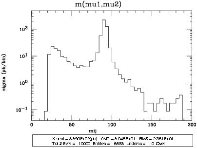
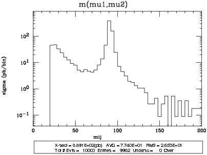
This means that we want histogram bins that are 4 GeV wide, and we want the axis to go from 0 to 200 GeV. Now, save the file and exit, and start the run. When done, inspect the invariant mass plot. You should be able to pick out the Z boson mass peak. Here's what it looks like at parton level (Madevent output):
and here's what it looks like after the events have been through the detector simulator Delphes: